Objectives
Central to optimisation are objectives, which in an abstract sense define the direction in which to steer the process of parameter refinement. The optimisation problem is defined as a weighted multi-objective optimisation, where each objective typically is associated with multiple data items itself. Each objective is scalarized, meaning that it is evaluated to a single scalar that represents its own cost or fitness. Each objective is assigned a weight, corresponding to its relative significance; weights are automatically normalised. Marler and Arora provide a good review on multi-objective optimisation [MOO-review].
The declaration of an objective establishes a way for a direct comparison between some reference data and some model data. With each pair of items from the reference and model data there is associated a weight, referred to as sub-weight that corresponds to the significance of this item relative to the rest of the items associated with an objective. These sub-weights are used in the scalarisation of the objective, and are also normalised.
Overview of Objectives Declaration
The declaration of an objective in the input file of SKPAR consists of the following elements:
objectives:
    - query: # a name selected by the end-user
        doc: "Doc-string of the objective (optional)"
        models:
            # Name of models having query_item in their database (mandatory)
        ref:
            # Reference data or instruction on obtaining it (mandatory)
        options:
            # Options for interpretation of reference/model data (optional)
        weight:
            # Weight of the objective (dflt: one)
        eval:
            # How to evaluate the objective (dflt: [rms, abserr]
An example of the simplest objective declaration – the band-gap of bulk Si in equilibrium diamond lattice – may look like that:
objectives:
    - Egap:
        doc: 'Si-diam-100: band-gap'
        models: Si.diam.100
        ref: 1.12
        weight: 5.0
        eval: [rms, relerr]
See also
Details of Objective Declaration
Query Label (query)
query is just a label given by the user. SKPAR does not interpret
these labels but uses them to query the model database in order to
obtain model data. Therefore, the only condition that must be met when
selecting a label is that the label must be available in the database(s)
of the model(s) that are listed after models.
It is the responsibility of the Get-Tasks to satisfy this condition. Recall that a get-task yields certain items (key-value pairs) in the dictionary that embodies the model database accessed as a destination of the task.
Certain get-tasks allow the user to define the key of the item, and
this key can be used as a query-label when declaring an objective.
Example of that is shown in Tutorial 1, where
the simple get_model_data task is used, and the query label
is yval.
Other tasks yield a fixed set of items – examples are the
get-tasks provided by the dftbutils package.
Please, consult their documentation to know which items are
available as query-labels: Available get-functions.
There is one case however, in which the above significance of
query is disregarded, and the specified label becomes irrelevant.
This is the case where the reference data of an objective is itself a
dictionary of key-value pairs (or results in such upon acquisition
from a file). This case is automatically recognised by SKPAR and the
user need not do anything special.
The query-label in this case can be something generic.
Example of such an objective can be found in
Tutorial 2, with queries labeled as
effective_masses or special_Ek.
Doc-string (doc)
This is an optional description – preferably very brief, which would
be used in reporting the individual fitness of the objective, and
also as a unique identifier of the objective (complementary to its
index in the list of objectives).
If not specified, SKPAR will assign the following doc-string automatically:
doc: "model_name: query_item".
Model Name(s) (models)
This is a single name, or a list of names given by the user, and is a mandatory field. A model name given here must be available in the model database. For this to happen, the model must appear as a destination of a Get-Task declaration (see Get Tasks).
Beyond a single model name and a list of model names, SKPAR supports also a list of pairs – [model-name, model-factor]. In such a definition, the data of each model is scaled by the model-factor, and a summation over all models is done, prior to comparison with reference data.
Therefore, the three (nonequivalent) ways in which models can be specified are:
objectives:
    - query:
        # other fields
        models: name   # or [name, ]
        # or
        models: [name1, name2, name3..., nameN]
        # or
        models:
            - [name1, factor1]
            - [name2, factor2]
            # ...
            - [nameN, factorN]
Reference Data (ref)
Reference data could be either explicitly provided, e.g.:
ref: [1.5, 23.4], or obtained from a file.
The latter gives flexibility, but is correspondingly more complicated.
Loading data from file is invoked by:
objectives:
    - query
        # other fields in the declaration
        ref:
            file: filename
            # optional
            loader_args: {key:value-pairs}
            # optional
            process:
                # processing options
SKPAR loads data via Numpy loadtxt() function, and the optional
arguments of this function could be specified by the user via
loader_args
Typical loader-arguments are:
unpack: True– transposes the input data; mandatory when loading band-structure produced fromdp_bandsorvasputilsdtype: {names: ['keys', 'values'], formats: ['S15', 'float']}– loads string-float pairs; mandatory when the reference data file consists of key-value pairs per line.
The process options are interpreted only for 2D array data (ignored
otherwise), and are as follows:
rm_columns: index, list_of_indices, or, range_specificationrm_rows: index, list_of_indices, or, range_specificationscale: scale_factor
NOTABENE: The indexes apply to the rows and columns of the file, and are therefore independent of the loader arguments (i.e. prior to potential transpose of the data). The indexes and index ranges are Fortran-style – counting from 1, and inclusive of boundaries.
Example:
objectives:
    - query:
      ...
      ref:
        file: filename
        process:
            rm_columns: 1                # filter k-point enumeration, and bands, potentially
            rm_rows   : [[18,36], [1,4]] # filter k-points if needed for some reason
            scale     : 27.21            # for unit conversion, e.g. Hartree to eV, if needed
      ...
Objective Weight (weight)
This is a scalar, corresponding to the relative significance of the objective compared to the other objectives. Objective weights are automatically normalised so that there sum is one.
Evaluation function (eval)
Each objective is scalarised by a cost function that can be optionally modified here. Currently only Root-Mean-Squared Deviation is supported, but one may choose whether absolute or relative deviations are used. The field is optional and defaults to RMS of absolute deviations.
objectives:
    ...
    - query:
        ...
        eval: [rms, abserr] # default, absolute deviations used
        # or
        eval: [rms, relerr] # relative devations
Options (options)
Options depend on the type of objective.
One common option is subweights, which allows the user to specify
the relative importance of each data-item in the reference data.
These sub-weights are used in the cost-function representing the
individual objective.
For details, see the sub-weights associated with different Reference Data And Objective Types below.
Reference Data And Objective Types
The format of reference data could be:
- single item: e.g. a scalar representing the band-gap of a semiconductor, or a reaction energy;
- 1-D array: e.g. the energy values of an energy-volume relation of a solid;
- 2-D array: e.g. the band-structure of a solid, i.e. the set of eigenstates at different k-number;
- key-value pairs: e.g. named physical quantities, like effective masses, specific E-k points within the first Brilloin zone, etc.
Declaring an objective for a single model is straight forward, and in this case a signle item reference data may be thought of as a special case of 1-D array. However, the distinction between the two makes sense if we want to construct an objective based on more than one models, as shown further below.
There are five types of objectives. The type is deduced from the combination of format of the reference data and number of model names. Therefore, SKPAR automatically distinguishes between the following five objectives types:
1) Single model, single item/1-D array reference data
This is the simplest objective type that associates one or more (1-D array) items with a query of one model.
In the case of an array reference data, one option is admitted: subweights.
The number of sub-weights must match the length of the reference data array.
Sub-weights are normalised automatically.
Example:
objectives:
    # single model, single scalar reference data
    - band_gap:
        ref: 1.12
        models: Si/bs

    # single model, 1-D array reference data
    - levels:
        ref: [-13.6, -5, -3.0]
        options:
            subweights: [1, 1, 2]
        models: molecule
2) Single model, 2-D array reference data
This objective type allows for greater flexibility in defining the association between individual reference and model data items, which may not be the trivial one-to-one correspondence between the entire arrays yielded by the query item.
The 2-D arrays (of reference and model data) are viewed as composed of bands – each row is referred to as a band, each column is referred to as a point. A visual representation of the concept is shown in Fig. 3.
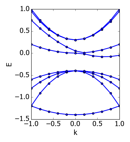
Fig. 3. Visual representation of a 2-D array in terms of bands. Each data item in the array is a circle on the plot. The lines represent the association of a row of data in the array with a band.
Correspondence between different bands of the model and reference data can be established via the following options:
use_ref: [...]use_model: [...]align_ref: [...]align_model: [...]
The use_ options admit a list of indexes, ranges, or a mix of indexes and
ranges – e.g. [[1, 4], 7, 9], and instruct SKPAR to retain only the
enumerated bands for the comparison of the resulting 2-D sub-arrays of
model and reference data.
Fortran-style indexing must be used, i.e. counting starts
from 1, and ranges are inclusive of both boundaries.
NOTABENE:
In any case, the final comparison (model vs reference) is over arrays of
identical shape, and the resulting arrays after the use_ clause should
be of the same shape.
The align_ options instruct SKPAR to subtract the value of a specific
data item in the array from all values in the array, i.e. change the
reference. This option admits a pair of band-index and point-index, or
a pair of band-index and a function name (min or max) to operate
on the indexed band. In either case, the value of the indexed data item or
the value returned from the function is subtracted from the model or
reference data prior to objective evaluation.
This objective type also admits subweights option, but in this case the
correspondence between sub-weights and data items needs more flexible
specification. This is to avoid the necessity of providing a full 2-D array
of sub-weight coefficients for each data item.
The following sub-options facilitate that:
objectives:
    ...
    - bands:
        ...
        options:
            ...
            subweights:
                dflt: 1.0
                values: [[[value range], subweight], ...]
                bands: [[[band-index range], subweight], ...]
Note
Correspondence between sub-weights and data, per data item, is established
after the application of use_ and align_ options have taken effect.
Example:
objectives:

    - bands:
        doc: Valence Band, Si
        models: Si/bs
        ref:
            file: ./reference_data/fakebands.dat #
            loader_args: {unpack: True}
            process:       # eliminate unused columns, like k-pt enumeration
                # indexes and ranges below refer to file, not array,
                # i.e. independent of 'unpack' loader argument
                rm_columns: 1                # filter k-point enumeration, and bands, potentially
                # rm_rows   : [[18,36], [1,4]] # filter k-points if needed for some reason
                # scale     : 1                # for unit conversion, e.g. Hartree to eV, if needed
        options:
            use_ref: [[1, 4]]                # fortran-style index-bounds of bands to use
            use_model: [[1, 4]]
            align_ref: [4, max]              # fortran-style index of band and k-point,
            align_model: [4, max]            # or a function (e.g. min, max) instead of k-point
            subweights:
                # NOTABENE:
                # --------------------------------------------------
                # Energy values are with respect to the ALIGNEMENT.
                # If we want to have the reference  band index as zero,
                # we would have to do tricks with the range specification
                # behind the curtain, to allow both positive and negative
                # band indexes, e.g. [-3, 0], INCLUSIVE of either boundary.
                # Currently this is not done, so only standard Fortran
                # range spec is supported. Therefore, band 1 is always
                # the lowest lying, and e.g. band 4 is the third above it.
                # --------------------------------------------------
                dflt: 1
                values: # [[range], subweight] for E-k points in the given range of energy
                # notabene: the range below is with respect to the alignment value
                    - [[-0.3, 0.], 3.0]
                bands: # [[range], subweight] of bands indexes; fortran-style
                    - [[2, 3], 1.5]   # two valence bands below the top VB
                    - [4 , 3.5]       # emphasize the reference band
        weight: 3.0
3) Single model, key-value pairs reference data
For this objective, a number of queries are made over a single model. The reference data is a dictionary of key-value pairs. Note that the name of the objective (meff below) has a generic meaning, and is not defining the query items. Instead, The queries are based on the keys from the reference data.
One options is admitted – subweights, and its value must be a dictionary
associating a weighting coefficient with a key.
One of the subweight-keys is dflt, allowing to specify a weight simultaneously
over all keys. The subweights are normalised automatically.
A key is excluded from the queries if its sub-weight is 0.
Example:
objectives:

    - meff:
        doc: Effective masses, Si
        models: Si/bs
        ref:
            file: ./reference_data/meff-Si.dat
            loader_args:
                dtype:
                # NOTABENE: yaml cannot read in tuples, so we must
                #           use the dictionary formulation of dtype
                    names: ['keys', 'values']
                    formats: ['S15', 'float']
        options:
            subweights:
                # consider only a couple of entries from available data
                dflt: 0.
                me_GX_0: 2.
                mh_GX_0: 1.
        weight: 1.5
4) Multiple models, single item reference data
All of the models are queried individually for the same query-item, and the result is scaled by the non-normalised model-weights or model factors, prior to performing summation over the data, to produce a single scalar. This scalar is seen as a new model data item. Accordingly, reference data is a single value too. This type of objective is convenient for expressing reaction energies as targets.
Example:
objectives:
    - Etot:
        doc: "heat of formation, SiO2"
        models:
            - [SiO2-quartz/scc, 1.]
            - [Si/scc, -0.5]
            - [O2/scc, -1]
        ref: 1.8
5) Multiple models, 1-D array reference data
A single query per model is performed, over several models. The dimension of the 1-D array of reference data must match the number of models.
The admitted option is
subweights– a list of floats, being normalised weighting coefficients in the cost function of the objective. This type of objective is convenient for expressing energy-volume relation as target, where the different models correspond to different volume.
Example:
objectives:
    - Etot:
        models: [Si/scc-1, Si/scc, Si/scc+1,]
        ref: [23., 10, 15.]
        options:
            subweights: [1., 3., 1.,]
REFERENCES
| [MOO-review] | R.T. Marler and J.S. Arora, Struct Multidisc Optim 26, 369-395 (2004), “Survey of multi-objective optimization methods for engineering” |