Tasks¶

SKPAR features dynamic model definition by the user, which greatly enhances its flexibility. The model is defined by a sequence of tasks, which represent the steps needed to obtaining model data. The tasks are declared in the input file and are executed in the given sequence at each iteration.

There are three task categories:

Set – model update – updates the model environment with the parameters generated by the optimiser at a given iteration;

Run – model execution – executes external programs, scripts or commands, to perform the necessary model calculations;

Get – collection of model data – acquire the relevant data from the various output files created during model execution.

Plot – plotting of objectives data (model and reference) – produce visual representation of objectives at each iteration; Plot-tasks are optional.

Refer to Fig. 2. Optimisation loop realised by SKPAR. for the corresponding steps in the optimisation flow.

The signature of each category and a brief usage is shown below.

For more complete examples see Tutorials.

NOTABENE:

Tasks should be entered as list items of the tasks: section in the input YAML file.

Set Tasks¶

tasks:
    - set: [parameter_file, work_directory, optional_templates]

Set-tasks serve to communicate the parameter values generated by the optimiser to the model.

The parameters (including iteration number and possibly parameter names) are written to parameter_file in work_directory, for which standard rules apply: ‘~’ is expanded to user directory, and if there is no path component included then it is relative to ‘.’. Default parameter file is current.par, and default work-directory is . if not explicitly specified.

The most important feature of the set task is its ability to update template files – optional_templates, according to the dictionary of parameters used in SKPAR. The following rules apply in this respect:

optinonal_templates is a filename or a list of filenames with the following structure: template.something or something.template.somthingelse;

template files must contain named place-holders which are substituted for the corresponding parameter values;

upon substitution, the output files bear the name of the template, except for the template. part being removed – for example: skdefs.template.py becomes skdefs.py;

templates are expected to be in work_directory, if they have no path component; else, standard path expansion applies;

place holders should be in the old string-formatting syntax for Python, i.e. %(parameter_name)parameter_type; NOTABENE: NO space after closing bracket!

Run Tasks¶

tasks:
    - run: [command, work_directory, input, output]

Run-tasks help to define model that must be optimised in a flexible way, depending on the specific problem without modifying SKPAR.

The mandatory command argument is a string or list of strings and may include options and arguments of an external executable, shell command, or a script.

The command is executed in work_directory, for which standard rules apply: ‘~’ is expanded to user directory, and if there is no path component included then it is relative to ‘.’. Default work-directory is ‘.’ if not explicitly specified.

The input and output files are optional and default to None and out.log in the working directory.

Run tasks support aliasing via the Executables section.

Get Tasks¶

tasks:
    - get: [get_function, source, destination, func_arguments]

Get-tasks serve to collect model data from source, optionally perform some analysis on it and put the result as a key-value item at the destination. The destination is an embodiment of the database of a model, which allows queries of the values corresponding to the available keys. (see Fig. 1. Conceptual block diagram of SKPAR. and Fig. 2. Optimisation loop realised by SKPAR.).

The signature of get-tasks shown above relies on a dictionary of known functions, which are mostly model-specific.

Available get-functions¶

The get_function must be one of those accessible to the user, as as listed in skpar/core/taskdict.py:

Generic
`get_model_data`	Generic routine based on `numpy.loadtxt()`
Specialised: DFTB+
`get_dftbp_data`	Get data resulting from a DFTB+ calculation, e.g. in detailed.out.
`get_dftbp_bs`	Get all data from DFTB+/dp_bands calculation of bandstructure.
`get_dftbp_meff`	Extract effective masses from DFTB+/dp_bands calculation of bandstructure.
`get_dftbp_Ek`	Extract named E-k points from DFTB+/dp_bands calculation of bandstructure.

Source and Destination¶

Beyond the mandatory get-function name, a get-task must have:

source (mandatory, string) – a directory name or a dictionary in the model database;

destination (optional, string) – a dictionary in the model database; source is tried if destination is not given, and a dictionary is automatically allocated in the database when a destination is first used in a get-task;

Optional Arguments¶

func_arguments (optional, dict) – a dictionary of key-value pairs, being keyword arguments of the get-function invoked. The possible arguments for each get-function can be checked via the table below, with links to the implementations underlying the available get-functions.

Plot Tasks¶

tasks:
    - plot: [plot_function, plot_name, list_of_objectives,
                optional_abscissa_key,
                optional_queries_list,
                kwargs]

Plot tasks produce .pdf plots with specified plot_name, visualising the reference and model data associated with an objective at each iteration. The filenames are tagged by an iteration number.

The data of the list_of_objectives is used as ordinate values. An objective is selected by a pair-list of [query_name, model_name], e.g. bands: Si. The abscissa values may be obtained via the optional_abscissa_key, or alternatively, the index numbers of individual data items are used. The optional_queries_list allows the plotting routine to obtain extra data produced by the model at each evaluation, by declaring a query within the plot-task. Obviously, both the abscissa key and the extra query keys must be present in the model database, and this must be guaranteed by the use of appropriate get-tasks.

The plot is realised by the plot_function, which should be selected from the table below (follow hyperlinks for details):

`plot_objvs`	generic plotting of 1D or 2D data
`plot_bs`	specialised routine to plot bandstructures

Plot-Task Examples:¶

Generic plot of a 1D array data:

tasks:
    ...
    # get both yval and xval from the model and put in poly3 database
    - get: [get_model_data, test_optimise/model_poly3_out.dat,  poly3, yval]
    - get: [get_model_data, test_optimise/model_poly3_xval.dat, poly3, xval]

    # plot yval of poly3 using xval of poly3 as abscissa key
    - plot: [plot_objvs, 'test_optimise/pdf/polyfit1', [[yval, poly3]], xval]

objectives:
    - yval:
        doc: 3-rd order polynomial values for some values of the argument
        models: poly3
        ref: [ 36.55, 26.81875, 10., 13.43125,  64.45 ]
        eval: [rms, relerr]

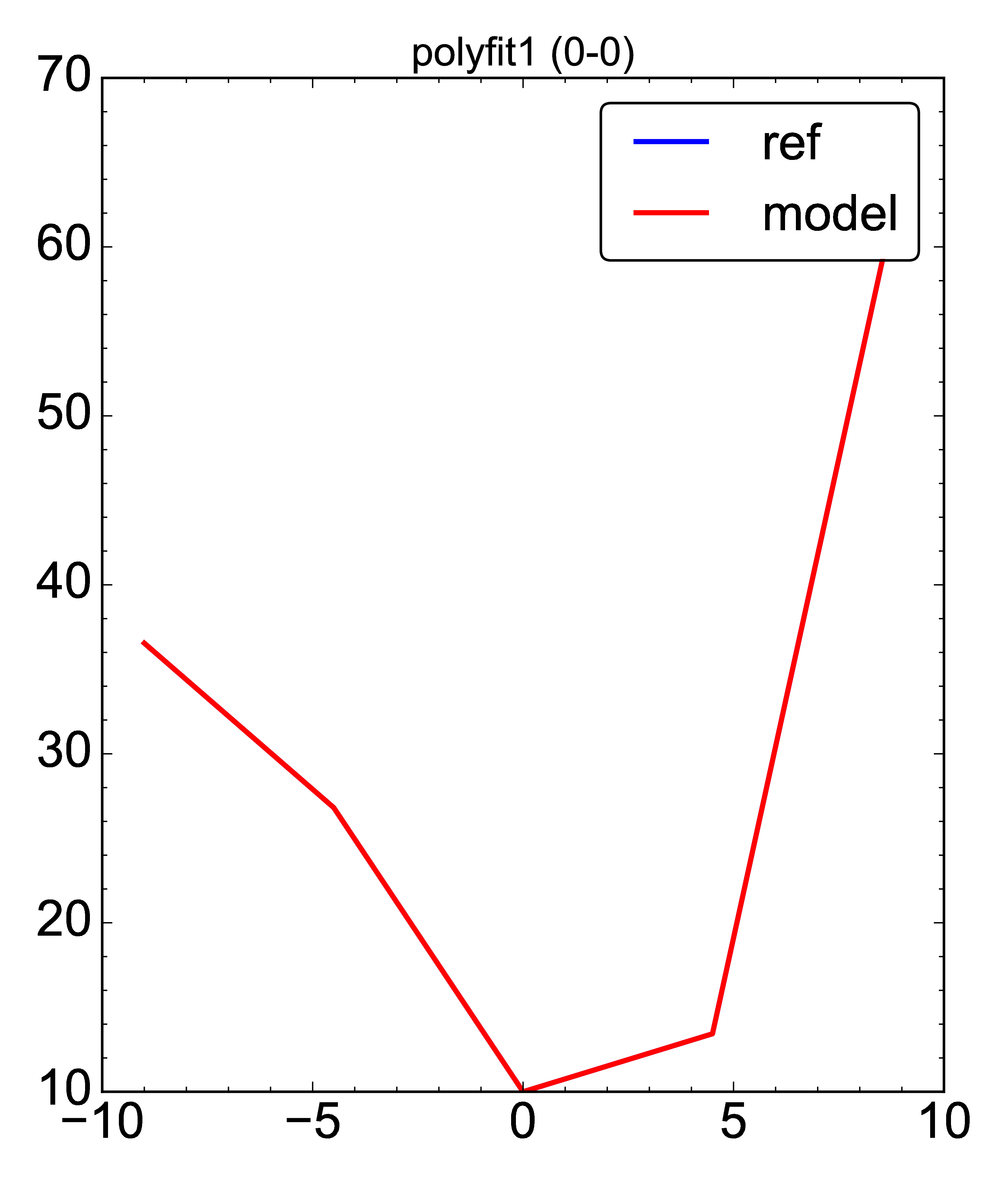
Fig. 4. 1-D array plotted with the generic ``plot_objvs`` function

Generic plot of a 2D array data.

This example plots a bandstructure (a fake one). Two problem with the resulting plot below is its integer x-axis, i.e. the k-line lengths are (generally) not correct, since k-point index is used as an abscissa; no labels either.

tasks:
    ...
    # load bands in fakemodel database; transpose input array after removing column 1
    - get: [get_model_data, reference_data/fakebands-2.dat, fakemodel, bands,
                    {loader_args: {unpack: True}, process: {rm_columns: [1]}}]
    # plot the bands using y-value index (along axis 1) as an x-value
    - plot: [plot_objvs, 'test_optimise/pdf/fakebandsplot', [[bands, fakemodel]]]

- bands:
    models: fakemodel
    ref:
        file: reference_data/fakebands.dat
        loader_args: {unpack: True}
        process:
            rm_columns: [1, 2, [8, 9]]

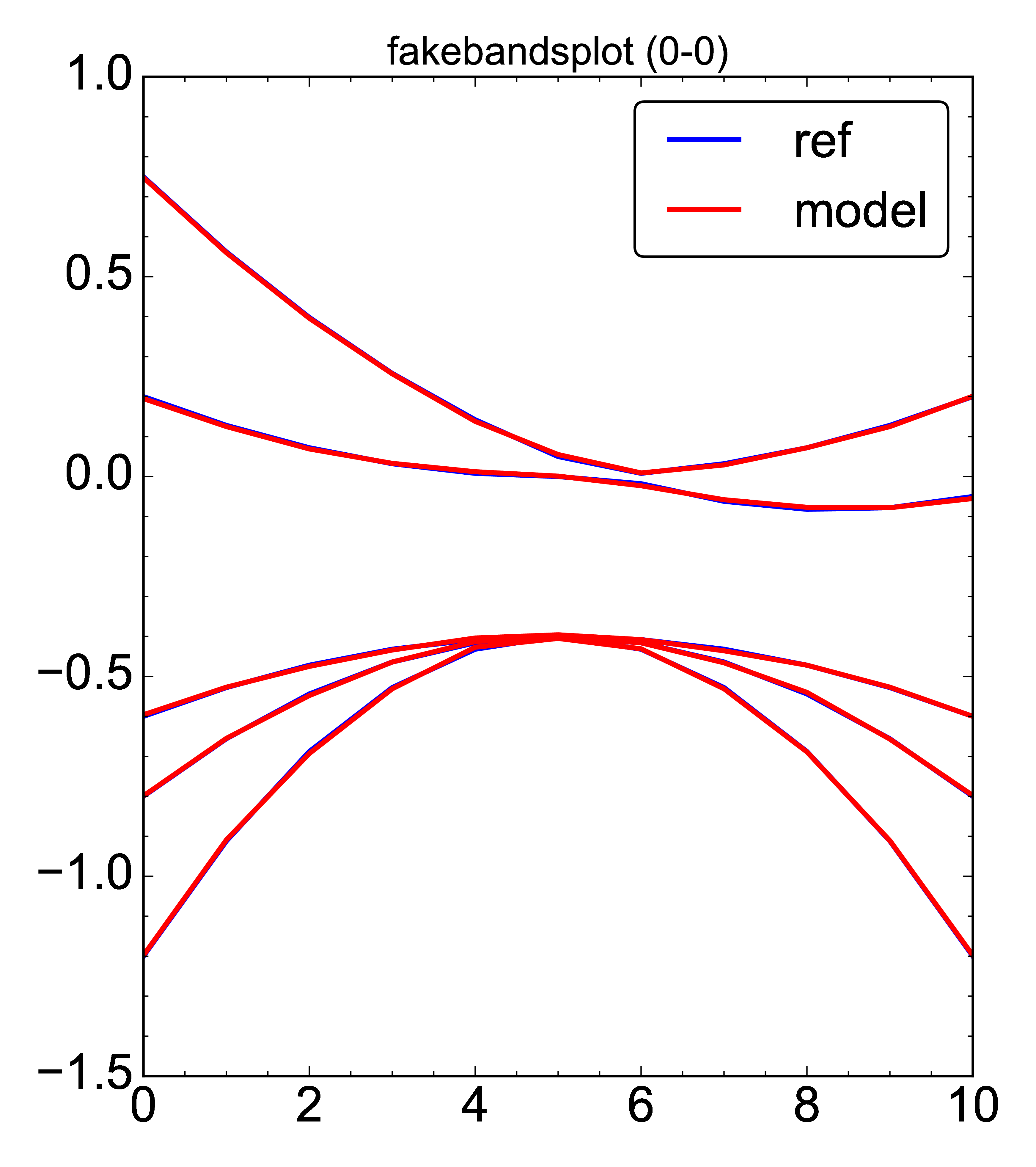
Fig. 5. 2-D array data plotted by the generic plot_objvs function

Specialised plot of a bandstructure.

This example plots a bandstructure properly. For this, the x-values are constructed and passed as an abscissa value. Moreover, it shows how to handle the case where the bandstructure information is split over three different objectives – we have one objective for the band-gap, another for the valence bands and yet another for the conduction band, and both VB and CB are 0-aligned. The magic here relies on:

strict definition of objectives with bands query: first VB, then CB

strict enumeration of objectives: fisrt Egap, then bands

tasks:
    ...
    # Get all data from DFTB+/dp_bands. This includes all needed for BS plot,
    # including 'Egap', 'bands', 'kticklabels'
    - get: [get_dftbp_bs, Si-diam/100/bs, Si.diam.100,
            {latticeinfo: {type: 'FCC', param: 5.431}}]

    # The plot_bs does magic when it sees the first objective being 'Egap'.shape==(1,)
    # it shifts the CB by the band-gap, so the band-structure is properly shown.
    # For this to happen, objectives declaration must be such that VB precedes CB!!!
    # The plot_bs will also show k-ticks and labels if requested, as below via
    # 'kticklabels'
    - plot: [plot_bs, Si-diam/100/bs/bs_2, [[Egap, Si.diam.100], [bands, Si.diam.100]],
                kvector, queries: [kticklabels]]

objectives:
    - Egap:
        doc: 'Si-diam-100: band-gap'
        models: Si.diam.100
        ref: 1.12
        weight: 5.0
        eval: [rms, relerr]

    - bands:
        doc: 'Si-diam-100: VALENCE band'
        models: Si.diam.100
        ref:
            file: ~/Dropbox/projects/skf-dftb/Erep fitting/from Alfred/crystal/DFT/di-Si.Markov/PS.100/band/band.dat
            loader_args: {unpack: True}
            process:
                rm_columns: 1      # filter k-point enumeration
        options:
            use_ref: [[1, 4]]                # Fortran-style index-bounds of bands to use
            use_model: [[1, 4]]
            align_ref: [4, max]              # Fortran-style index of band-index and k-point-index,
            align_model: [4, max]            # or a function (e.g. min, max) instead of k-point
        eval: [rms, relerr]

    - bands:
        doc: 'Si-diam-100: CONDUCTION band'
        models: Si.diam.100
        ref:
            file: ~/Dropbox/projects/skf-dftb/Erep fitting/from Alfred/crystal/DFT/di-Si.Markov/PS.100/band/band.dat
            loader_args: {unpack: True}
            process:
                rm_columns: 1      # filter k-point enumeration
        options:
            use_ref: [5, 6]                # fortran-style index enumeration: NOTABENE: not a range here!
            use_model: [5, 6]              # using [[5,6]] would be a range with the same effect
            align_ref: [1, 9]              # fortran-style index of band and k-point, (happens to be the minimum here)
            align_model: [1, min]          # or a function (e.g. min, max) instead of k-point
        eval: [rms, relerr]

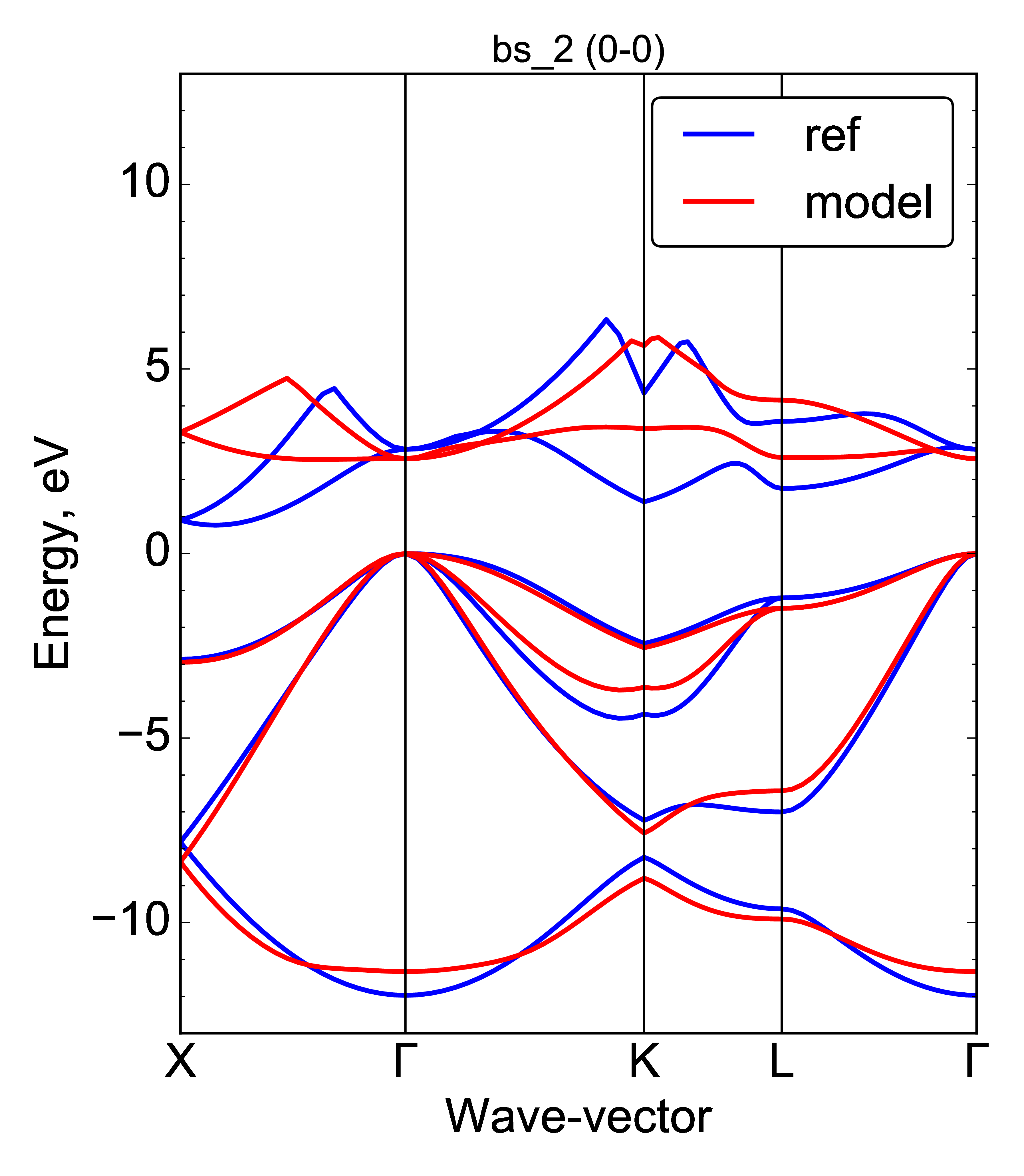
Fig. 6. Band-structure plotted by the ``plot_bs`` function